
Open source, open data, open course
We recently had the third instalment of the course in Throughput Sequencing technologies and bioinformatics analysis. This course aims to provide students, as well as users of the organising service platforms, basic skills to analyse their own sequencing data using existing tools. We teach both unix command line-based tools, as well as the Galaxy web-based framework.
I coordinate the course, but also teach a two-day module on de novo genome assembly. I keep developing the material for this course, and am increasingly relying on material openly licensed by others. To me, it is fantastic that others are willing to share material they developed openly for others to (re)use. It was hugely inspiring to discover material such as the assembly exercise, and the IPython notebook to build small De Bruijn Graphs (see below). To me, this confirms that ‘opening up’ in science increases the value of material many orders of magnitude. I am not saying that the course would have been impossible without having this material available, but I do feel the course has become much better because of it.
‘Open’ made this course possible
This course used:
- openly available sequencing data released by the sequencing companies (although some of the Illumina reads are behind a – free – login account)
- sequencing data made openly available by individual researchers
- code developed for teaching made available by individual researchers under a permissive license
- open source software programs
(for a full list or resources, see this document).
I am extremely grateful to the authors/providers of these resources, as they greatly benefitted this course!
Thanks to:
‘Opening up’ is the least I can do to pay back
In exchange, the very least I can do is making my final course module openly available as well.
The rest of this post describes the material and it’s sources in more detail.
Assembly exercise
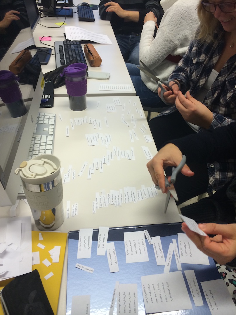
Here I used the excellent tool developed by Titus Brown to generate ‘reads’ from a piece of text. I started with a text based on a quote I found online, and modified it to add a few more repeated regions. Students received ~5x coverage in reads of 14 characters (spaces were replacers with underscores) and were asked in groups of 4 to 5 students to reconstruct the original text. I’ve added this part two years ago and it is a great way to start the module. Not only is there a lot of student activity, each group comes up with strategies that are aspects of algorithms actually used in programs for de novo assembly. Some cut out the reads with scissors, find overlapping ones and physically build the ‘ladder’. Others use a text editor for this, and put the consensus sequence below. Students keep track of reads they already used. Some start at multiple sections, or draw connections between the reads. Usually, at least one group googles the first part they reconstruct, find the original text and do ‘reference guided assembly’ (they often think they’re done, at which point I ask them to check the online version with the reads they were given).

Different approaches for the assembly exercise
Playing around with small De Bruijn Graphs
This part I added this year. Reusing the very useful python code generated by Ben Langmead for his computational genomics classes, I made an IPython notebook where students could build small de Bruijn Graphs at different kmer sizes. This showed them how longer kmers resolve repeats, as well as that too long kmers reduce overlaps between reads. Also, the graphs were excellent to demonstrate the effect of single-base errors in reads (build a graph based on 5 identical reads, add one read with a single base change in the middle to visualise that many new nodes are added to the graph because of this). Check out the results here.

De Bruijn Graph of the sequence “GCTGATCGATTT” at k = 3
Assembly using Velvet
The structure of this part was developed by Nick Loman when he came over to help me teach the very first instance back in 2011. Students run velvet on MiSeq reads released by Illumina, each with their own kmer size, and the resulting N50s are plotted against kmer size in a google spreadsheet (see this year spreadsheet here). This graph builds over time and beautifully shows how the N50 peaks at a certain kmer. Then paired end information and mate pairs (also released by Illumina) are added.
Assembly using HGAP or SPAdes
The course ran on a Thursday and the following Monday. This enabled me to ask the students to start a long-running assembly at the end of day 1 (we had 2 CPUs and about 32GB RAM per student). Students could choose to assembly a pure PacBio dataset (from the company) with HGAP, or a combined Illumina paired end + Oxford Nanopore MinION dataset with SPAdes. The MinION data was released by Nick Loman et al shortly before the course started, making this the first course to use actual MinION data for a hands-on practical.
Assembly evaluation
Students mapped reads back to the assemblies using bwa and visualised alignments in the IGV genome browser. Quality was assessed with REAPR, which also indicated where it thought the assembly should be broken due to conflicts with the mate pair data. Students visually inspected the regions indicated by REAPR and were asked to decide whether they agreed with the program. This part was deliberately ran without the reference genome, although this was available. I wanted to teach the students how to perform validation in the absence of a ground-truth reference (given more time, I would have probably repeated this part with the reference).
